


Trajectory Optimization using Direct Collocation
(part 4 in Cart-Pole series)


Welcome back, let's get started.
We've discovered the surprising power of the Linear Quadratic Regulator (LQR), but it also has its limits. LQR has a basin of attraction around the point we've linearized the dynamics around. If the cart-pole is in a state outside of this basin, the system becomes unstable and the controller goes mad. To save our pendulum from these horrible nonlinear dynamics, we need to swing it back to our stable basin using some sort of swing-up algorithm. That's where trajectory optimization comes into the picture.
I came across trajectory optimization after reading Daniel Piedrahita's article about cart-pole control. To learn more about this topic and more I've been watching Dr. Russ Tedrake's lectures from the course MIT 6.832 - Underactuated Robotics. I've also watched Dr. Matthew Kelly's introductory video to trajectory optimization and read his paper on how to implement direct collocation. All of these sources are fantastic and I highly recommend you take a look at them!
What is trajectory optimization?
LQR is a closed-loop control algorithm that spans the entirety of state space. Put simply, anywhere you are, the controller can manage to get you back to a stable fixed point. However, this only works for linear dynamics which require linearization. Trajectory optimization is an open-loop solution to control which can be useful for specific tasks, such as creating a swing-up trajectory. Instead of having a solution for the entire state space, trajectory optimization only creates a trajectory that we need to follow. After we're back in our basin of attraction, we can switch on LQR again!
Trajectory optimization, as the name suggests, uses optimization to minimize the cost of control for a specific trajectory. An optimization problem works by trying to minimize the value of a function called the objective function. This function is dependent on decision variables that need to fulfill some constraints. The decision variables for these types of problems are often the state and control signals, x and u, and how long the trajectory takes to finish. Using notation from Matthew Kelly, trajectory optimization can be described in what's known as the Lagrange form:
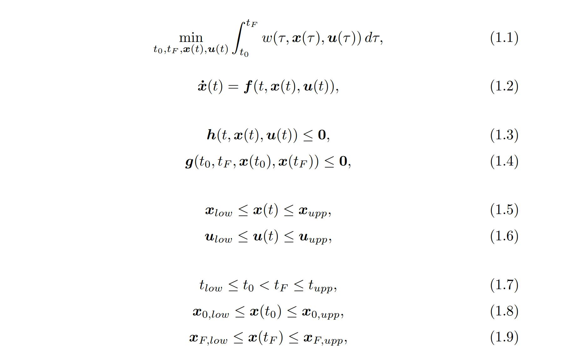
The objective function (1.1) tries to minimize w which is the integrand of the trajectory. This problem is subject to the system dynamics (1.2) but also constraints along the path (1.3). This could for example be that a car avoids pedestrians on its way to the goal. There are also boundary constraints (1.4) that put constraints on the initial and final states. The state and control signal also have bounds (1.5)(1.6), for instance, max speeds, voltages, etc. Finally, the initial and final states and time have some limits (1.7)(1.8)(1.9).
Direct Collocation
One trajectory optimization algorithm is called direct collocation. The direct part means that the problem is discretized, often into what's called a nonlinear program, or NLP, which is what we will do. Converting a trajectory optimization problem into an NLP problem is known as transcription, and direct collocation falls under the umbrella of so-called direct transcription methods.
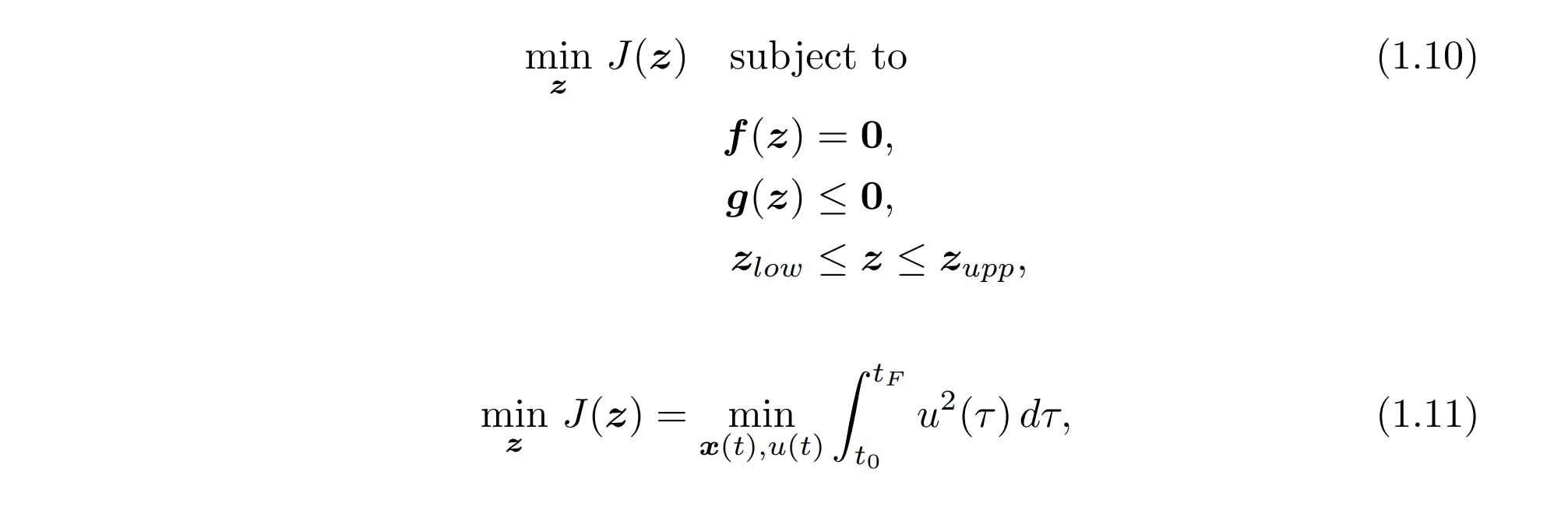
Nonlinear programs can be generalized as (1.10) an objective function J of some decision variables z with some equality constraints f, inequality constraints g and bounds on z. The dynamics constraint (1.2) is an equality constraint while the others are inequality constraints. An easy objective function to implement is the integral of the control signal squared (1.11). We can do this if we regard the control signal as a scalar function. This makes sense for the cart-pole where the control is the motor voltage. This objective function, therefore, tries to create a smooth trajectory with a minimized control input.
Trapezoidal Collocation
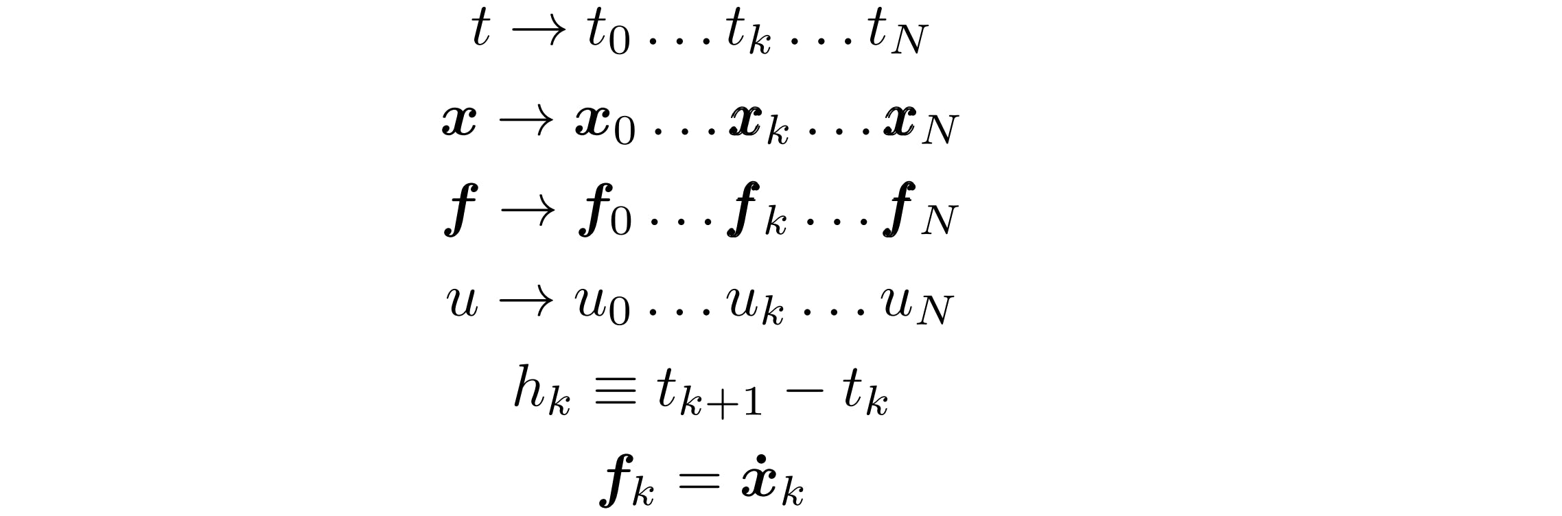
We still haven't discretized our NLP. To do this, there are again several options to choose from. An easy method to implement is called trapezoidal collocation. We begin by discretizing the decision variables into values at discrete points in time. These are called collocation points and there can be an arbitrary N of them which are separated in time by the time step h. Here f denotes the dynamics.
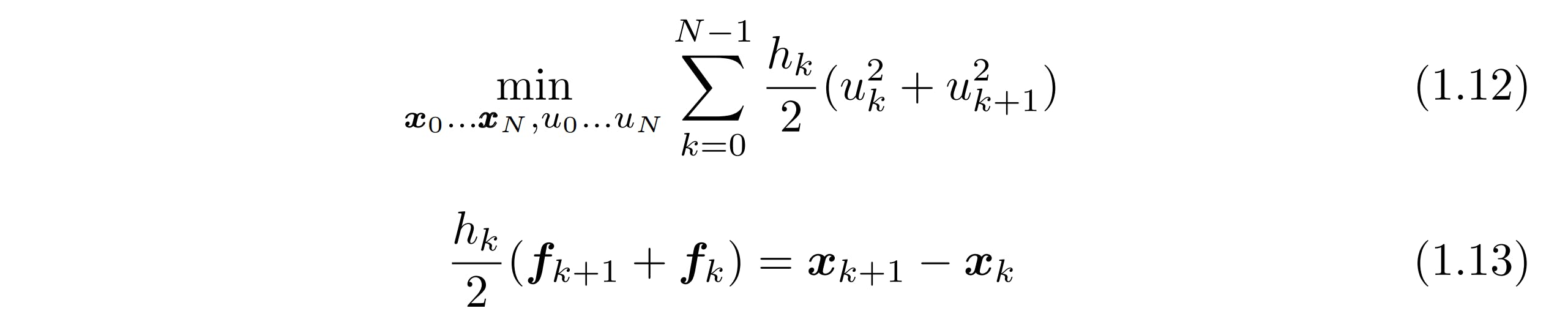
I won't delve into the proof that trapezoidal collocation accurately approximates the continuous dynamics. Instead, the discretized objective function has been provided below (1.12) as well as the discretized equality constraint on the dynamics (1.13).
If we add in the constraints on the initial and final state as well as their bounds and put this into a solver, this should produce a solution! All that's missing is an initial guess of the trajectory for the solver to optimize. An easy guess to make is just to interpolate from the initial state to the final state with the control signal being zero, and this dumb guess is often enough for the solver to come up with an actual solution!
Spline
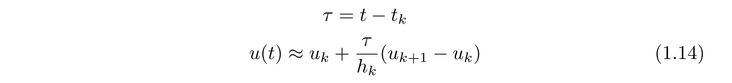
After your solver has come up with a solution for the optimization problem, it spits out a sequence of length N of the optimal state and control signal. These N collocation points need to be converted back into a continuous function. The control signal can be easily converted using piecewise linear interpolation. Mathematically, the functions between the points can be constructed using the equation below (1.14).
The state is a bit harder as it can be converted using quadratic interpolation. Instead of connecting the collocation points with lines, points are connected by quadratic functions. Interpolation using low-degree polynomial functions is called spline interpolation. These functions can be constructed using the equation below (1.15).

The Code
Now we have all the tools we need to start coding! We will create a class that takes in the dynamics, constraints and the number of collocation points N. The libraries used are numpy and parts of scipy for the solver minimize and the cubic interpolator CubicSpline.
import numpy as np
from scipy.optimize import minimize
from scipy.interpolate import CubicSpline

class DirectCollocation():
    def __init__(self, N: int, dynamics, N_states: int, N_controls: int, state_lower_bound, state_upper_bound, control_lower_bound, control_upper_bound, tolerance=1e-6):
        self.N = N
        self.dynamics = dynamics
        self.N_states = N_states
        self.N_controls = N_controls

        self.state_lower_bound = state_lower_bound.T[0]
        self.state_upper_bound = state_upper_bound.T[0]
        self.control_lower_bound = control_lower_bound.T[0]
        self.control_upper_bound = control_upper_bound.T[0]
        self.tolerance = tolerance
The constraints consist of the lower and upper bounds of the state and control variables. These are flipped to row vectors for easy manipulation. Besides those parameters, there's also the number of state variables N_states, the number of control variables N_controls and the tolerance. N_states and N_controls are useful for calculations. The tolerance specifies how accurate the solver should be; A lower tolerance means a high accuracy.
Next up is the method make_guess which makes the initial guess. This takes in the initial_state and the desired final_state and makes a linear interpolation between those two. The initial guess of the control is zero through the entire trajectory.
    def make_guess(self, initial_state, final_state):
        self.initial_state = initial_state.T[0]
        self.final_state = final_state.T[0]

        self.initial_variables = np.hstack([
            np.hstack([np.linspace(initial, final, self.N) for initial, final in zip(self.initial_state, self.final_state)]),
            np.zeros(self.N_controls*self.N),
        ])
        return self.initial_variables

    def variables_to_state_control(self, variables):
        state = variables[:self.N_states*self.N]
        control = variables[self.N_states*self.N:(self.N_states+self.N_controls)*self.N]
        return state, control
I also threw in the method variables_to_state_control since this is important when it comes to using a solver. The solver can only use data in the form of a row vector, so all of the decision variables (state and control) need to be packed into this single vector. The initial guess, self.initial_variables, is created in this way and variables_to_state_controls takes in the decision variables from the solver and unpacks them into the state and control.
Up next is the objective_function. As the math (1.11) implies, this spits out the quadratic cost of the control signal which the solver tries to minimize.
    def objective_function(self, variables):
        state, control = self.variables_to_state_control(variables)
        result = 0
        for i in range(self.N_controls):
            for k in range(self.N-1):
                result += (self.h/2)*(control[self.N*i+k]**2+control[self.N*i+k+1]**2)
        return result
The constraints can be categorized as either equality constraints or inequality constraints. In code, these are packed up similarly to the decision variables as row vectors. For the equality constraints, the solver ensures that the elements of this vector are always zero. The equality constraints are created in the method eq_constraints. These consist of the constraints on the initial and final state and the dynamic constraints along the trajectory.
    def eq_constraints(self, variables):
        state, control = self.variables_to_state_control(variables)
        constraints = []

        for k in range(self.N_states):
            constraints.append(state[self.N*k]-self.initial_state[k])
            constraints.append(state[self.N*k+self.N-1]-self.final_state[k])

        state_current = state[0::self.N]
        control_current = control[0::self.N]
        dynamics_current = self.dynamics(np.vstack(state_current), np.vstack(control_current)).T[0]

        for k in range(self.N-1):
            state_next = state[k+1::self.N]
            control_next = control[k+1::self.N]
            dynamics_next = self.dynamics(np.vstack(state_next), np.vstack(control_next)).T[0]

            dynamic_constraint = state_next-state_current-self.h/2*(dynamics_next+dynamics_current)
            constraints.extend(list(dynamic_constraint))

            state_current = state_next
            control_current = control_next
            dynamics_current = dynamics_next

        return constraints
The inequality constraints are created in the method ineq_constraints. The solver ensures that the elements of this vector are never zero. For now, these are the upper and lower bounds of the variables.
    def ineq_constraints(self, variables):
        state, control = self.variables_to_state_control(variables)
        constraints = []

        for k in range(self.N):
            current_state = state[k::self.N]
            current_control = control[k::self.N]

            constraints.extend(list(np.array(current_state)-self.state_lower_bound))
            constraints.extend(list(self.state_upper_bound-np.array(current_state)))
            constraints.extend(list(np.array(current_control)-self.control_lower_bound))
            constraints.extend(list(self.control_upper_bound-np.array(current_control)))

        return constraints
Finally, the optimal control is solved using make_controller. This method takes in the duration of the trajectory, the number of points to interpolate N_spline, the initial_state and the desired final_state. It first creates an initial guess of the trajectory. The constraints are packed into a dictionary that the solver can process. The solver itself uses Sequential Least Squares Programming (SLSQP) and takes in the objective function, initial guess, constraints and tolerance and spits out a solution of both the state and control signals. If N_spline is defined, then the state and control are splined and interpolated respectively.
    def make_controller(self, time, initial_state, final_state, N_spline=None):
        self.time = time
        self.N_spline = N_spline
        self.h = (self.time)/self.N

        self.make_guess(initial_state, final_state)
        constraints = [
            {"type": "eq", "fun": self.eq_constraints},
            {"type": "ineq", "fun": self.ineq_constraints},
        ]

        sol = minimize(
            fun=self.objective_function,
            x0=self.initial_variables,
            method="SLSQP",
            constraints=constraints,
            tol=self.tolerance
        )
        state, control = self.variables_to_state_control(sol.x)
        N_time = np.linspace(0, time, self.N)

        if N_spline:
            N_spline_time = np.linspace(0, time, N_spline)

            state_spline = np.vstack([
                CubicSpline(N_time, s_row)(N_spline_time) for s_row in state.reshape((self.N_states, self.N))
            ])
            control_spline = np.vstack([
                np.interp(N_spline_time, N_time, c_row) for c_row in control.reshape((self.N_controls, self.N))
            ])
        else:
            state_spline, control_spline = np.vstack(state), np.vstack(control)

        return state_spline, control_spline
Simulation
Using our code for direct collocation, we can now plan a swing-up trajectory for a single pendulum. We then use this control signal and when the pendulum is close to the upper fixed point, we switch on our LQR controller. This was simulated using 41 collocation points and a trajectory duration of 1 second. And... go
Let's try it with two pendulums! To make our LQR way more stable, we'll make the outermost pendulum way lighter than the other one. Let's set the duration to 2 seconds and use 61 collocation points.
Issues
So, as you can see above, the trajectory planner doesn't always work out, but why is that? Well, the devil's in the details.
The integrator of the direct collocation algorithm is slightly different from the Rk4. The small differences in the dynamics, and that there isn't a collocation point for every time step, paired with the chaotic nature of the double pendulum make the trajectory unstable.
Another issue is the calculation time. The single pendulum took 17 seconds to calculate. The double pendulum however took a whopping 7.5 minutes!
There are ways of fixing this. For the stability issues, we can use a time-varying LQR controller that stabilizes the dynamics along the trajectory. We can also use Model-Predictive Control, or MPC, which calculates a new trajectory for every time step to compensate for the inaccuracies. This however requires a fast calculation time which can be accomplished by using a faster solver and/or programming language. But for now, this is promising!
Next up
I'll try to look into Kalman filters again. It would also be interesting to find a better solver and make a faster trajectory planner so that MPC can be implemented. Making a time-varying LQR controller would also be cool!
Regarding the physical cart-pole, the motor driver I have wasn't powerful enough so I've ordered a new one from AliExpress which should arrive shortly.