

Controlling the Cart-Pole using LQR
a good first step controller (part 3 in Cart-Pole series)


Hi! Today's topic: Full-state feedback control. What is it? How do we optimize it? Can we do better? On the bullet-point list of new things: linearization, minimizing cost and LQR.
By the way, if you want to have a deeper look into the code, visit the GitHub repository! https://github.com/sackariaslunman/inverted-pendulum
Linearizing the Cart-Pole
Controlling the cart-pole will not be easy; the system has non-linear dynamics. Worse yet, when you add more poles to the cart, the dynamics also become chaotic. Most basic controllers (that I have a sliver of knowledge in designing) operate with linear dynamics. To use a linear controller on a non-linear system you need to approximate dynamics in a way that makes them linear.
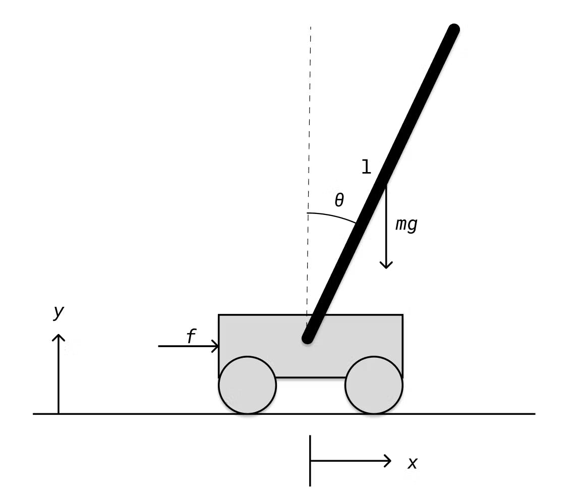
To do this we can make some assumptions about our system, starting with that when we start our controller, we let go of the pole in the upright position, i.e. the angle θ is 0. We also assume then assume that our controller will be able to control this well so that the cart's velocity dx and the angular velocity dθ are 0. We also assume that the cart starts at some arbitrary position x which we also set to 0.
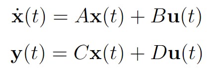
Using our new initial conditions it is now possible to approximate the linear dynamics at this specific point, where x, dx, θ and dθ are all 0, using a method called linearization. Since we used x to denote the cart's position I will denote the full state as a bold x. In its non-linear form x changes based on a non-linear function f that depends on the current state and a control signal vector u.
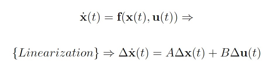
Using linearization, the approximated linear dynamics can be described using a matrix A that describes how each variable changes based on itself and the other variables in the full state. Each variable also changes based on u which is described in the B matrix. Here I've denoted the linearized full-state and control vector as Δx and Δu respectively. So how do we calculate A and B?
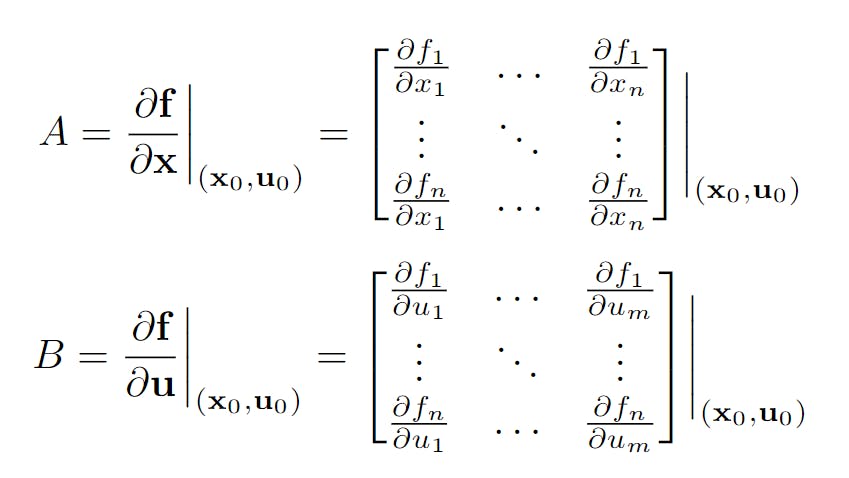
As you can see, it's quite a handful to do by hand, especially when you have many states; the number of elements has complexity O(n^2) where n is the number of states. Basically, the A and B matrices together describe the "tangent" of how the state variables change at a specific state x0 and control state u0.
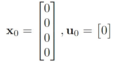
In our case, x0 should be chosen to be where the pole is balanced, i.e. the upright position where all variables are 0. Likewise, when the pole is balanced the control signal shouldn't need to fire so u0 is also 0.
And this is just the case with one pole! Luckily, I've already calculated these matrices for an arbitrary number of poles. I'm not going to show the final equations since they are disgustingly huge.
Control using Full-State Feedback
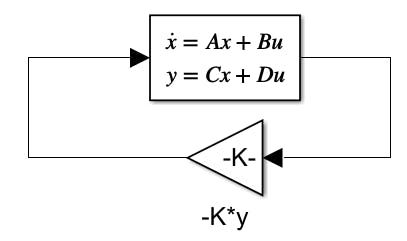
So, how do we control a system that is described using a linear state space model? That's where the Full-State Feedback, or FSFB, regulator comes in. It is ridiculously simple; way simpler than PID controllers if you've played around with those. I watched Christoper Lum's lecture on FSFB control and I can happily recommend the entire series of lectures.
To make the most basic type of FSFB regulator, we need to assume that every variable in our state is observable. The observable variables can be described as a subset of x called y and their dependence on u. I've omitted the deltas in the figure below.
In our case, C becomes the identity matrix of size n by n where n is the number of variables in our state. For our system, the observable state does not depend on the control so D becomes 0, or more specifically, a column vector of size n by 1 where all elements are 0.
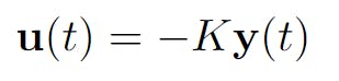
Finally, using this knowledge we can design our regulator. Since we can observe every variable at each time step, if we can set a proportional gain for each variable, and the system is controllable, then we can control the entire state. Yes, that's it. Just a proportional gain that we will call K. We will design our control u to be equal to -K*y.
Optimal control relies heavily on the concepts of system controllability and observability. It's not the goal of this article to explain those concepts but I've provided some links. You can also watch Christopher Lum's lectures.
Optimizing the FSFB regulator using LQR
After modeling our FSFB regulator we are left with one question: how do we optimize the gain K? This is where LQR, or the Linear-quadratic regulator, comes in. LQR tries to optimize K based on how "costly" the different variables in our state are. For our cart-pole, a costly variable might be θ. We might want to make this 0 as fast as possible and worry about the other variables later. Using LQR, we can specify that θ is more costly than the others and then optimize our controller based on these criteria.
K is optimized using the above equation. The costs of the different state variables are specified on the diagonal of the diagonal matrix Q. The costs of the control signals are likewise specified in the R matrix in the same manner.
As you can see, K is not included in the equation. To solve for K you use something called the continuous-time algebraic Ricatti equation or CARE. You can look it up if you want but in Python, it can be solved by using SciPy and NumPy.
import numpy as np
from scipy.linalg import solve_continuous_are

S = solve_continuous_are(A, B, Q, R) # S is the solution for CARE
K = np.linalg.inv(R) @ B.T @ S # how to calculate K using S
And that's it, two rows of code! Pretty simple if you ask me.
Implementing the controller
To implement controllers in Python there's already a library that you can use called python-control which I highly recommend. However, since I want to learn all of this from scratch, I've opted for making my own Full-state Feedback regulator class called FSFB. You can have a look at the code below.
from scipy.signal import cont2discrete
import numpy as np

class FSFB:
    def __init__(self, A, B, C, D, dt: float):
        self.A = A
        self.B = B
        self.C = C
        self.D = D
        self.dt = dt

        self.discretize()

    def discretize(self):
        dlti = cont2discrete((self.A,self.B,self.C,self.D),self.dt)
        self.A_d = np.array(dlti[0])
        self.B_d = np.array(dlti[1])
What I haven't yet explained is discretization and the discretize method. Since our computers work with zeros and ones, we have to adapt our linear model to work in discrete time rather than continuous time. The function cont2discrete takes in A and B (as well as C and D, but they stay the same after discretization) and calculates their discrete counterparts A_d and B_d based on the time step dt.
I've also made a subclass of FSFB called LQR that implements a method that calculates the gain K called K_lqr using CARE and its discrete counterpart using DARE. There's also the method calculate_K_r which calculates the gain K_r which lets the controller follow a reference signal r, which I won't go into detail about in this article. Finally, the feedback methods take in the current state and reference signal and calculate the next control signal.
from scipy.linalg import solve_continuous_are, solve_discrete_are

class LQR(FSFB):
    def calculate_K_lqr(self, Q, R):
        self.Q = Q
        self.R = R
        S = solve_continuous_are(self.A, self.B, Q, R)
        S_d = solve_discrete_are(self.A_d, self.B_d, Q, R)

        self.K_lqr = np.linalg.inv(R) @ self.B.T @ S
        self.K_lqr_d = np.linalg.inv(R + self.B_d.T @ S_d @ self.B_d) @ (self.B_d.T @ S_d @ self.A_d)

    def calculate_K_r(self):
        K_r = np.true_divide(1, self.D + self.C @ np.linalg.inv(-self.A + self.B @ self.K_lqr) @ self.B)
        K_r[K_r == np.inf] = 0
        K_r = np.nan_to_num(K_r)
        self.K_r = K_r.T

        K_r_d = np.true_divide(1, self.D + self.C @ np.linalg.inv(np.eye(self.A_d.shape[0]) - self.A_d + self.B_d @ self.K_lqr_d) @ self.B_d)
        K_r_d[K_r_d == np.inf] = 0
        K_r_d = np.nan_to_num(K_r_d)
        self.K_r_d = K_r_d.T

    def feedback(self, state, r):
        u = self.K_r @ r - self.K_lqr @ state
        return u

    def feedback_d(self, state, r):
        u_d = self.K_r_d @ r - self.K_lqr_d @ state
        return u_d
Regulating the Cart-Pole
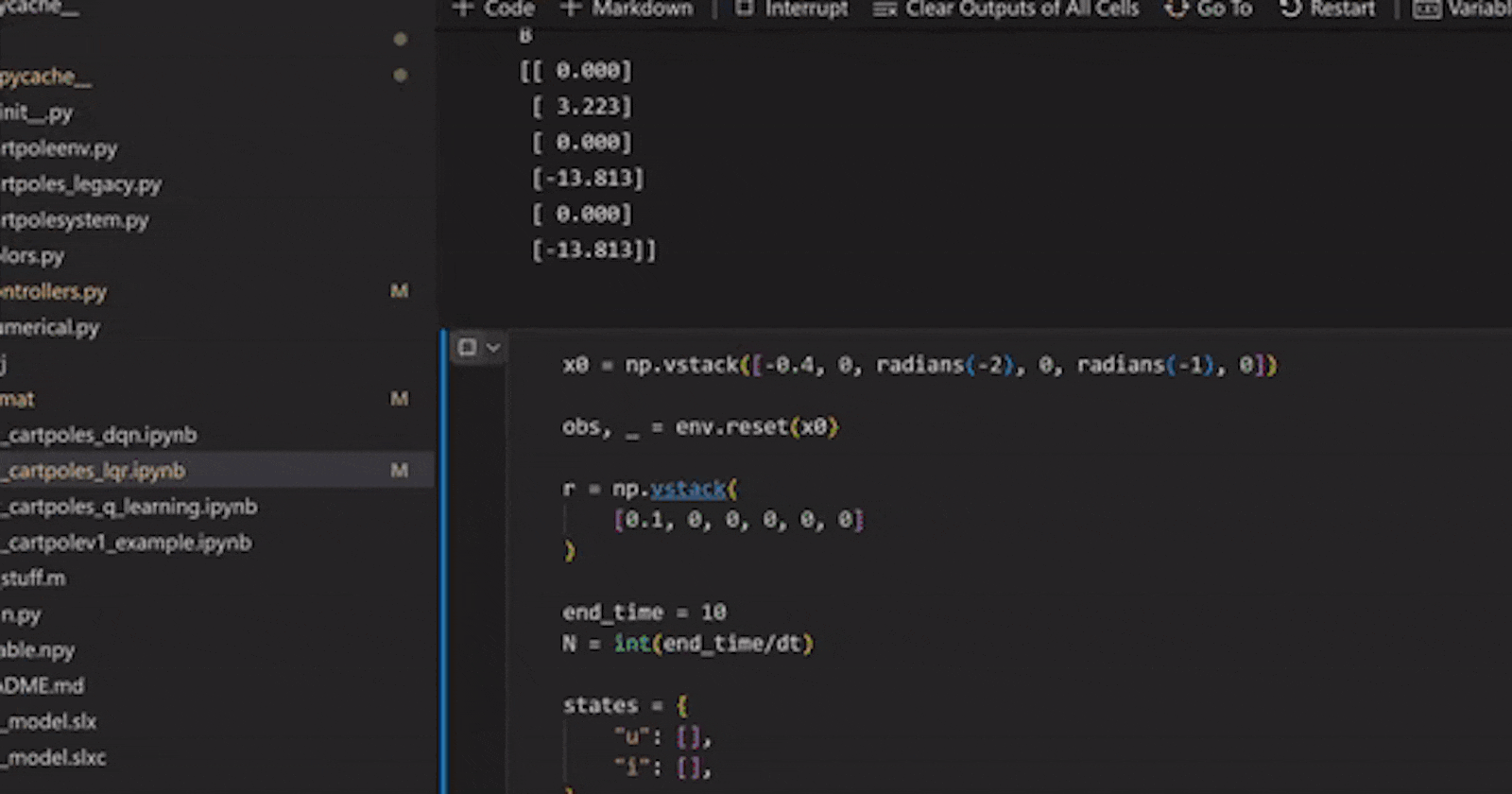
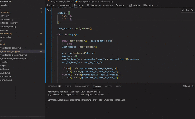
Finally! Using the environment that we set up in the last article and our new LQR class we can now regulate the cart-pole. I'm using a Q with ones on the diagonal and R containing a single element 0.1 for Va. The initial conditions are x = -0.4, dx = 0, θ = 45° and dθ = 0. The reference signal, or goal, is x = 0.1, dx = 0, θ = 0° and dθ = 0. And... go!
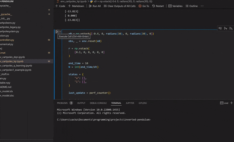
Woohoo! Let's add another pole. Adding another pole makes the system even more unstable so the starting angles for both poles will be 30° to ensure that our controller can regulate the system. And... go!
Flaws
LQR works great if you can measure all state variables accurately. In real life, this is almost certainly impossible. There's always some noise in the system dynamics and measurements, and often you can't measure the entire state. That's where the Kalman filter and LQG control come in which we will have a look at next time.
We are also regulating an unrealistic system. Right now, the motor draws upwards of 2400 Watts: not ideal. To simulate a more realistic system, a good idea could be to do some system identification on the physical model when that has been built. But for now, we'll have to stick with the current system parameters.
Next up
I'll look into implementing a Kalman filter and combining it with LQR control to create an LQG controller. I've also read Daniel Piedrahita's article where he talks about regulating a cart-pole using exciting stuff like LQR-Trees and trajectory planning which I will have a look at later on!
Also, the motor driver for the physical model has arrived, so I'll get busy building that too!