The Cart-Pole is a classic problem in dynamical systems and control theory. The goal is for a controller to balance an inverted pendulum (or several) on top of a cart by moving the cart backward and forwards, violently swinging the pole around until it stays still.

I'm currently trying to build a physical model of this system and balance it using different control methods. To do this the proper way, I'll first need to model the system to optimize my controller and simulate the controlled system to verify that it works as intended, so let's do that.

Mathematical modeling

Forget about the coding; first, we need to model the system. The Cart-Pole system is what's known as a nonlinear dynamic system. To begin visualizing the system in our heads, let's imagine a cart and just one pole.

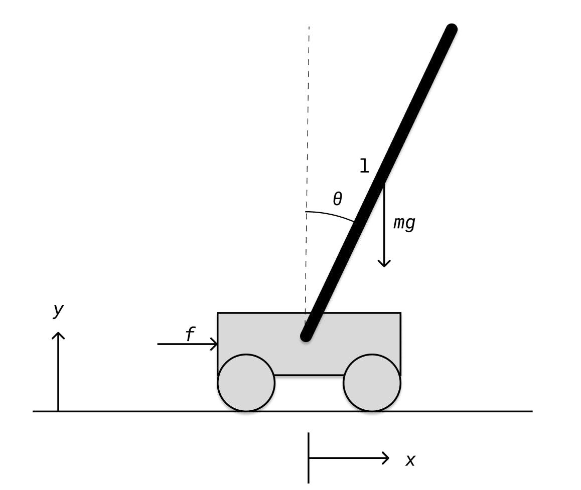
The cart can move along the horizontal axis or the x-axis. It can not move along the vertical axis or the y-axis. The pendulum is attached to the cart along the middle and can rotate freely in the xy-plane. The angle between the pendulum and the y-axis is a function of time and will be denoted as θ. Likewise, the cart's position on the x-axis is x. The pole has a length of l and a mass of m that exerts a gravitational force. There's also an input force f which our controller uses to balance the pole.

All forces aren't written out. Two of the missing forces are the friction between the cart and the track which is proportional to the cart's velocity and the friction in the pole's rotation joint.

The system can be mathematically described by the use of several different methods such as Newton's laws of motion or the Lagrangian. Since this is a popular and well-documented model in mechanics I will save myself some work by using Colin D. Green's [1] solution for the equations which can be found here. The equations describe a generalized cart-pole system with multiple poles indexed by i.

Now we can add as many poles as we please, but the model is not complete yet. The physical cart will be fastened to a timing belt that will be driven by a DC motor. The DC motor sits on the x-axis and can be described by two equations.

Since the inductance of small DC motors is very small it has been excluded from our equations.

Now, our DC motor's output shaft is coupled with a timing belt on which our cart sits. Therefore, the velocity and acceleration of the cart are proportional to the angular velocity ω and angular acceleration at the output shaft respectively by the radius of the output shaft, r. Likewise, the output torque TL is proportional to the input force f at the cart by r. Using this information we can reformulate equations (3) and (4) in terms of derivations of x, f and r.

Now we can get the final equation for the cart's acceleration by inserting equations (5) and (6) into (1).

Coding the system

With the power of these two equations, we can now begin coding the system in Python. Heads up, the coding was quick and dirty and needs to be refactored; I just wanted to get a simulator out quickly.

Let's begin with the pole. Let's make it a class whose constructor takes in the mass m, initial angle angle0, length l, coefficient of friction u_p and an optional pendulum pole which is attached to the end of this one. It also takes in a color that it will display in the visual part of the simulator. Then we initialize the states of the pole as a dictionary state where the keys are the named variables and the values are lists of the variable values through time. We also have some imports for typing and not having to type math.sin and math.cos .

from __future__ import annotations
from math import sin, cos

class Pole:
    def __init__(
        self, 
        mass: float, 
        angle0: float, 
        length: float, 
        pole_friction: float, 
        color: tuple[int,int,int], 
        child: Pole | None
        ):

        self.m = mass
        self.l = length
        self.u_p = pole_friction
        self.color = color  

        self.state = {
            "theta": [angle0],
            "d_theta": [0],
        }

        self.child = child

Next up is an update method that updates the states of the system. The arguments are the time step dt, the acceleration of the cart dd_x and the gravitational acceleration g. The algorithm calculates the angular acceleration of the pole dd_theta by use of equation (2) and uses the forward Euler method to calculate the angular velocity d_theta and finally the angle theta. We then save the new states and append them to the state lists.

    def update(self, dt: float, dd_x: float, g: float):
        theta = self.angle()
        d_theta = self.angular_velocity()

        dd_theta = 3/(7*self.lh())*(g*sin(theta)-dd_x*cos(theta)-self.u_p*d_theta/(self.m*self.lh()))
        d_theta = d_theta + dd_theta * dt
        theta = theta + d_theta * dt

        self.state["d_theta"].append(d_theta)
        self.state["theta"].append(theta)

We also make use of some helper methods. One of these is the __iter__() method which puts the pole and all of its attached poles into a list that can be iterated through. We also have two methods that return the angle or angular acceleration at a specific time step, with the default being the last value. Finally the lh() method just returns the length of the pole.

    def lh(self):
        return self.l/2

    def __iter__(self):
        poles = [self]
        pole = self.child
        while pole:
            poles.append(pole)
            pole = pole.child
        return iter(poles)

    def angle(self, t=None):
        if not t:
            t = len(self.state["theta"])-1
        return self.state["theta"][t]

    def angular_velocity(self, t=None):
        if not t:
            t = len(self.state["d_theta"])-1
        return self.state["d_theta"][t]

    def __str__(self):
        return f"Pole:\n  Mass: {self.m}\n  Length: {self.l}\n  Friction: {self.u_p}\n  Child: {self.child is not None}"

Moving on we have the cart. Similarly, it has a constructor that takes in all parameters and initializes the state. Two of these parameters are a minimum position min_x and a maximum position max_x which are the boundaries of the track. It also takes in a pole, or rather a chain of poles, and a DC motor which we haven't written yet.

class Cart:
    def __init__(
        self, 
        mass: float, 
        cart_friction: float, 
        x0: float, min_x: float, 
        max_x: float, 
        color: tuple[int,int,int], 
        motor: DCMotor, 
        pole: Pole
        ):

        self.m = mass
        self.u_c = cart_friction
        self.min_x = min_x
        self.max_x = max_x
        self.color = color

        self.motor = motor

        self.state = {
            "x": [x0],
            "d_x": [0],
            "dd_x": [0]
        }

        self.pole = pole

    def __iter__(self):
        return iter(self.pole)

    def total_mass(self):
        M = self.m
        for pole in self:
            M += pole.m
        return M

    def x(self, t=None):
        if not t:
            t = len(self.state["x"])-1
        return self.state["x"][t]

    def velocity(self, t=None):
        if not t:
            t = len(self.state["d_x"])-1
        return self.state["d_x"][t]

    def acceleration(self, t=None):
        if not t:
            t = len(self.state["dd_x"])-1
        return self.state["dd_x"][t]

The update method of the cart calculates dd_x by use of equation (7) and has dt, input voltage Va and g as arguments. With the forward Euler method, we calculate the velocity d_x and position x, but if the position is beyond the boundaries min_x or max_x, we clamp it to the nearest boundary. It then iterates through the chain of poles and updates every one of them. Finally, we also update the state of the motor.

    def update(self, dt: float, Va: float, g: float):
        x = self.x()
        d_x = self.velocity()
        M = self.total_mass()

        sum1 = sum([pole.m*sin(pole.angle())*cos(pole.angle()) 
            for pole in self])
        sum2 = sum([pole.m*pole.lh()*pole.angular_velocity()**2
            *sin(pole.angle()) for pole in self])
        sum3 = sum([pole.u_p*pole.angular_velocity()
            *cos(pole.angle())/pole.lh() for pole in self])
        sum4 = sum([pole.m*cos(pole.angle())**2 for pole in self])

        dd_x = (g*sum1-7/3*((1/self.motor.r**2)*(self.motor.K/self.motor.Ra
            *(Va*self.motor.r-self.motor.K*d_x)-self.motor.Bm*d_x)+sum2
            -self.u_c*d_x)-sum3)/(sum4-7/3*(M+self.motor.Jm/self.motor.r**2))
        d_x = d_x + dd_x * dt
        x = self.clamp(x + d_x * dt)

        self.state["dd_x"].append(dd_x)
        self.state["d_x"].append(d_x)
        self.state["x"].append(x)

        for pole in self:
            pole.update(dt, dd_x, g)
        self.motor.update(dt, d_x)

    def clamp(self, x: float):
        if x > self.max_x:
            return self.max_x
        elif x < self.min_x:
            return self.min_x
        return x

Lastly, the DC motor. I won't go into detail more than that it has the simplest code. Since we are only interested in its angular velocity omega and angular acceleration d_omega at the moment, most of the state updating happens in the cart and therefore the update method for the motor is very concise.

class DCMotor:
    def __init__(
        self, 
        resistance: float, 
        K: float, 
        inertia: float, 
        friction: float, 
        radius: float, 
        color: tuple[int,int,int]
    ):

        self.Ra = resistance
        self.K = K
        self.Jm = inertia
        self.Bm = friction

        self.color = color
        self.r = radius

        self.state = {
            "omega": [0],
            "d_omega": [0]
        }

    def angle(self, t=None):
        if not t:
            t = len(self.state["omega"])-1
        return self.state["omega"][t]

    def angular_velocity(self, t=None):
        if not t:
            t = len(self.state["d_omega"])-1
        return self.state["d_omega"][t]

    def update(self, dt, d_x):
        d_omega = d_x / self.r
        omega = self.angle() + d_omega * dt

        self.state["d_omega"].append(d_omega)
        self.state["omega"].append(omega)

A quick-and-easy simulator

All we have to do now is initialize the parameters of our system, i.e. the cart, motor and poles, and give them some initial states.

cart = Cart(0.5, 0.05, 0, -0.8, 0.8, colors.red,
    DCMotor(0.05, 0.5, 0.05, 0.01, 0.05, colors.black),
    Pole(0.2, 10/180*pi, 0.2, 0.005, colors.green, 
        Pole(0.2, 5/180*pi, 0.15, 0.005, colors.blue, 
            Pole(0.2, 15/180*pi, 0.15, 0.005, colors.purple, None
            )
        )
    )
)

Here we've created a triple-pole system. Each pole has a mass of 0.2 kg and a coefficient of friction at the joint of 0.005. The poles decrease in length from 0.2 m to 0.15 m to 0.1 m and have colors green, blue and purple. They have initial angles of 10°, 5° and 15°, written in radians.

The cart is red and has a mass of 0.5 kg and a coefficient of friction between it and the track of 0.05. It starts at x=0 on the track and can travel from x=-0.8 m to x=0.8 m. The track, therefore, has a length of 1.6 m.

To simulate the system, we simply have to run a loop where we update the cart. To visualize this, I've made a bad stupid ugly simulator in PyGame. I'm not going to go over this code but you are free to try it out.

import sys, pygame
from time import perf_counter
from math import pi, sin ,cos
from cartpole import Cart, Pole, DCMotor
pygame.init()

size = width, height = 1200, 600

screen = pygame.display.set_mode(size)

class Colors:
    red = (255,0,0)
    green = (0,255,0)
    blue = (0,0,255)
    purple = (255,0,255)
    cyan = (0,255,255)
    yellow = (255,255,0)
    black = (0,0,0)
    white = (255,255,255)
    gray = (100,100,100)
colors = Colors

dt = 0.001
g = 9.81

cart = Cart(0.5, 0.05, 0, -0.8, 0.8, colors.red,
    DCMotor(0.05, 0.5, 0.05, 0.01, 0.05, colors.black),
    Pole(0.2, 10/180*pi, 0.2, 0.005, colors.green, 
        Pole(0.2, 5/180*pi, 0.15, 0.005, colors.blue, 
            Pole(0.2, 15/180*pi, 0.10, 0.005, colors.purple, None
            )
        )
    )
)

def si_to_pixels(x: float):
    return int(x * 500)

last_update = 0
start_time = perf_counter()
i = 0

font = pygame.font.Font('freesansbold.ttf', 20)

while True:
    current_time = perf_counter()-start_time
    if current_time > dt + last_update:
        last_update = current_time
    else:
        continue

    for event in pygame.event.get():
        if event.type == pygame.QUIT: 
            sys.exit()

    screen.fill(colors.gray)

    cart.update(dt, 12*cos(i*dt*2), g)

    x0 = si_to_pixels(cart.x()) + width//2
    y0 = height//2
    pygame.draw.rect(screen, cart.color, (x0, y0, 20, 10))

    max_x = width//2 + si_to_pixels(cart.max_x)
    min_x = width//2 + si_to_pixels(cart.min_x)
    pygame.draw.rect(screen, cart.color, (min_x-10, y0, 10, 10))
    pygame.draw.rect(screen, cart.color, (max_x+20, y0, 10, 10))

    motor_x0 = min_x-100
    motor_sin = si_to_pixels(sin(-cart.motor.angle())*0.05)
    motor_cos = si_to_pixels(cos(-cart.motor.angle())*0.05)

    pygame.draw.polygon(screen, cart.motor.color, [
        (motor_x0+motor_sin, y0+motor_cos),
        (motor_x0+motor_cos, y0-motor_sin),
        (motor_x0-motor_sin, y0-motor_cos),
        (motor_x0-motor_cos, y0+motor_sin),
    ])

    x0 += 10
    for pole in cart:
        x1 = x0 + si_to_pixels(pole.l * sin(pole.angle()))
        y1 = y0 + si_to_pixels(-pole.l * cos(pole.angle()))
        pygame.draw.line(screen, pole.color, (x0, y0), (x1, y1), 10)
        x0 = x1
        y0 = y1

    texts = [
        f"Time: {round(i*dt,2)} s",
        f"",
        f"Cart:",
        f"Position: {round(cart.x(),2)} m",
        f"Velocity: {round(cart.velocity(),2)} m/s",
        f"Acceleration: {round(cart.acceleration(),2)} m/s^2",
        f"",
        f"Motor:",
        f"Angle: {round(cart.motor.angle(),2)} rad",
        f"Angular velocity: {round(cart.motor.angular_velocity(),2)} rad/s",
    ]

    for k, text_k in enumerate(texts):
        text = font.render(text_k, True, colors.black, colors.gray)
        text_rect = text.get_rect()
        screen.blit(text,(0,(text_rect.height)*k,text_rect.width,text_rect.height))

    pygame.display.flip()
    i += 1

Concisely, we update the state of the system every 1 ms and then draw out the different subsystems. The boundaries are marked by red squares and the motor is a square that spins in place. We also write out some data in the top-left corner. The input voltage 12*cos(i*dt*2) is a cosine function of time that makes the cart move backward and forwards repeatedly.

And there we go, all done!

Flaws

A big flaw in the system is that we are using the forward Euler method for numerical integration. This isn't as accurate as other methods, especially with a larger time step. In the future, I'll probably use some Runge-Kutta method instead, but I need to do some research first. Using a time step that is too big also makes the system go unstable. For my simulator, the system goes unstable with a time step greater than around 0.03.

Future

I've ordered all of the parts for the real physical model that I'm building. Until they arrive, I will continue developing the model and simulator. The model is incomplete as it does not include any gear ratio between the motor and timing belt.

The simulator is still very ugly and badly written. I plan to remake the simulator and convert it into an OpenAI gym environment so that it is easy to use for training a reinforcement learning model. Next up is doing just that and perhaps writing a simple controller for balancing a single pole.

Next part - Making a Cart-Pole test environment

References

[1] Green, Colin D. (2020) Equations of Motion for the Cart and Pole Control Task.
[link1]