

Making a Cart-Pole test environment
using RK4 integration and gym (part 2 in Cart-Pole series)


Happy new year! The thumbnail is a simulation of a system first studied by Edward Lorenz aptly named the Lorenz attractor, or the butterfly attractor. It's the namesake of the famous butterfly effect and gave rise to chaos theory. This brings us to today's topic of numerical integrators since it's very important to have one of high quality to be able to accurately simulate chaotic systems, such as a double inverted pendulum.
A new system model
So, the old model with a Cart, Pole and Motor class worked well with the forward Euler method where integrating is easy. However, for higher-quality integration schemes, it helps to have the full state of your system and just one function that differentiates it, otherwise, it gets messy quickly.
The new model is just a single class called CartPoleSystem which represents the entire system: cart, poles and motor. The constructor takes in a cart and motor, represented as tuples, and a list of poles, represented as a list of tuples. It also takes in the gravitational acceleration g and the integration scheme represented as a string. We will return to the different kinds of integrators and how we implement them.
from __future__ import annotations
import numpy as np
from numpy import sin, cos, pi
color = tuple[int,int,int]

class CartPoleSystem:
    def __init__(
        self,
        cart: tuple[float, float, float, float, float, color],
        motor: tuple[float, float, float, float, float, float, float, color],
        poles: list[tuple[float, float, float, float, color]],
        g: float,
        integrator: str = "rk4"
    ):
        self.cart = np.array(cart[:-1], dtype=np.float32)
        x0, m, u_c, min_x, max_x, cart_color = cart
        self.m = m
        self.u_c = u_c
        self.min_x = min_x
        self.max_x = max_x
        self.cart_color = cart_color

        self.motor = np.array(motor[:-1], dtype=np.float32)
        Ra, Jm, Bm, K, r, min_Va, max_Va, motor_color = motor
        self.Ra = Ra
        self.Jm = Jm
        self.Bm = Bm
        self.K = K
        self.r = r
        self.min_Va = min_Va
        self.max_Va = max_Va
        self.motor_color = motor_color

        self.num_poles = len(poles)
        self.poles = np.array([pole[:-1] for pole in poles], dtype=np.float32)
        self.pole_colors = [pole[-1] for pole in poles]
        self.M = self.m + sum(mp for (_, mp, _, _) in self.poles)
        self.g = g

        self.integrator = integrator

        self.reset(self.get_initial_state())

    def reset(self, initial_state):
        self.state = np.array([
            initial_state
        ])
        self.d_state = np.array([
            np.zeros(len(initial_state))
        ])

    def get_initial_state(self):
        return np.hstack([np.array([self.cart[0], 0, 0]), np.hstack([[angle0, 0] for angle0 in self.poles.T[0]])])
The constructor saves all of the named parameters and the cart, motor and poles as NumPy arrays. The get_initial_state method gets the initial state based on the passed parameters to the constructor. This state is then passed to the reset method which adds it to the first row of the state matrix. We also have the d_state matrix which stores the calculated derivative of the state at each time step. The full state with n poles is as follows:
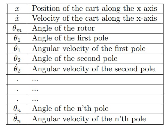
To get the next state, we need to differentiate the current state. The differentiate method does pretty much what the update methods of the previous codebase did, except for the full state in just one function.
    def differentiate(self, state, u):
        Va = u[0]
        sum1 = sum([m*sin(state[3+k*2])*cos(state[3+k*2]) for k,(_,m,_,_) in enumerate(self.poles)])
        sum2 = sum([m*(l/2)*state[3+k*2+1]**2*sin(state[3+k*2]) for k,(_,m,l,_) in enumerate(self.poles)])
        sum3 = sum([(u_p*state[3+k*2+1]*cos(state[3+k*2]))/(l/2) for k,(_,_,l,u_p) in enumerate(self.poles)])
        sum4 = sum([m*cos(state[3+k*2])**2 for k,(m,_,_,_) in enumerate(self.poles)])

        d_x = state[1]
        dd_x = (self.g*sum1-(7/3)*((1/self.r**2)*((self.K/self.Ra)*(Va*self.r-self.K*d_x)-self.Bm*d_x)+sum2-self.u_c*d_x)-sum3)/(sum4-(7/3)*(self.M+self.Jm/(self.r**2)))
        d_theta_m = d_x / self.r

        dd_thetas = np.hstack([[state[3+k*2+1],(3/(7*l/2)*(self.g*sin(state[3+k*2])-dd_x*cos(state[3+k*2])-u_p*state[3+k*2+1]/(m*l/2)))] for k,(_,m,l,u_p) in enumerate(self.poles)])
        return np.hstack([d_x, dd_x, d_theta_m, dd_thetas])
The code is messy and could be refactored, but for now, it works. The differentiated state is returned in the following format:
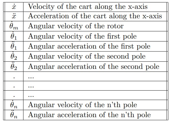
The system is brought forward in time with the step method. This method gets the current state and then differentiates and integrates it either using the forward Euler method or RK4 (I promise I will explain what this is later) which spits out the next state. It then constrains/clamps the next state to within its maximum/minimum boundaries and appends it and the current state's derivative to the state matrices.
    def get_state(self, t=-1):
        return self.state[t]

    def step(self, dt: float, Va: float):
        state = self.get_state()
        next_state, d_state = None, None

        if self.integrator == "fe":
            next_state, d_state = fe_step(dt, self.differentiate, state, [Va])
        else:
            next_state, d_state = rk4_step(dt, self.differentiate, state, [Va])
        next_state = self.clamp(next_state)

        self.update(next_state, d_state)

        return next_state

    def clamp(self, state):
        x = state[0]
        if x > self.max_x:
            x = self.max_x
        elif x < self.min_x:
            x = self.min_x
        state[0] = x

        for k in range(self.num_poles):
            state[3+k*2] %= 2*pi

        return state

    def update(self, next_state, d_state):
        self.state = np.vstack([self.state, next_state])
        self.d_state = np.vstack([self.d_state, d_state])
Besides these important methods, we also have two helper methods that will be used later in the environment class.
    def max_height(self) -> float:
        return sum(l for _,_,l,_ in self.poles)

    def end_height(self) -> float:
        state = self.get_state()
        return sum(l*cos(state[3+k*2]) for k, (_,_,l,_) in enumerate(self.poles))
Numerical integration using RK4
What exactly is numerical integration? Without going too heavy into math lingo, a numerical integrator is a function that receives a state and how to calculate its derivative and then tries to predict what the next state will be. We already touched on this with the forward Euler method which is a numerical integrator, just not a very good one. To brush up on the topic I can recommend watching a series of lectures by professor Steve Brunton on Differential Equations and Dynamical Systems that delves into numerical integration.
The problem with the forward Euler method, or FE, is that it tends to overshoot, and the overshooting only increases with a bigger time step. This can even lead to the simulated system becoming unstable when the time step increases over a certain threshold. This threshold depends on the system and how "dynamic" it is.
The Runge-Kutta methods are methods for numerical integration that try to be more accurate than FE using the same time step. Brunton has a great explanation of the 2nd-order and 4th-order Runge-Kutta methods which you can find here. In my simulation I'm using the 4th-order Runge-Kutta method or RK4. I won't go into details about the algorithm and why it works; it has to do with trying to eliminate the errors of the derivative's Taylor series expansion.
Code
My implementation of FE and RK4 both receive a time step, the differentiation function, the state and the control state. They then calculate the next state using the derivative of the current state.
def fe_step(dt: float, differentiate, x0, u):
    d_x = differentiate(x0, u)
    x = x0 + dt * d_x
    return x, d_x

def rk4_step(dt: float, differentiate, x0, u):
    f1 = differentiate(x0, u)
    f2 = differentiate(x0 + (dt/2) * f1, u)
    f3 = differentiate(x0 + (dt/2) * f2, u)
    f4 = differentiate(x0 + dt * f3, u)

    d_x = f1 + 2*f2 + 2*f3 + f4
    x = x0 + (dt/6) * d_x
    return x, d_x
Flaws
RK4 is great, but it's not enough for chaotic systems like our cart-pole system. It let me increase the time step from 0.02 to 0.025 without the system going unstable, but that was it. Chaotic systems typically need more powerful and tailor-made integration schemes. I might come back and find a better integrator than RK4.
Gym environment
OpenAI has an open-source package called Gym that is used for testing one's machine learning models on some predefined dynamic models. Gym already has a cart-pole environment, but this is an idealized version with only a single pole and no friction or motor. However, Gym also lets you define your own environment which is what we will do.
The environment is defined as a class called CartPolesEnv and is a subclass of Gym's Env class. The constructor takes in a CartPoleSystem, the time step dt and g. It initializes the screen, its size and the font that will be used for the rendering. Then, more importantly, it initializes the action space or control space. This object defines the minimum and maximum values, as well as the data type and shape, of our control signals, which in our case is the input voltage Va. We do the same for our observation space which is our full state. The class Box is used for creating spaces of continuous signals. If discrete signals are preferred then there's also the Discrete class.
from numpy import radians, pi, sin, cos
from random import uniform
import gym
from gym import spaces
import numpy as np
from cartpolesystem import CartPoleSystem
import pygame
from time import perf_counter

class CartPolesEnv(gym.Env):
  def __init__(
    self,
    system: CartPoleSystem,
    dt: float,
    g: float,
  ):

    super(CartPolesEnv, self).__init__()
    self.system = system
    self.max_height = system.max_height()
    self.dt = dt
    self.g = g

    self.screen: pygame.surface.Surface | None = None
    self.font: pygame.font.Font
    self.i : int
    self.width = 1200
    self.height = 700
    self.size = self.width, self.height

    self.action_space = spaces.Box(
      low=system.min_Va,
      high=system.max_Va,
      dtype=np.float32
    )

    num_of_poles = system.num_poles

    obs_lower_bound = np.hstack([np.array([system.min_x, np.finfo(np.float32).min]), np.tile(np.array([0.0, np.finfo(np.float32).min]), num_of_poles)])

    obs_upper_bound = np.hstack([np.array([system.max_x, np.finfo(np.float32).max]), np.tile(np.array([2*pi, np.finfo(np.float32).max]), num_of_poles)])

    self.observation_space = spaces.Box(
      low=obs_lower_bound,
      high=obs_upper_bound,
      shape=(2+2*num_of_poles,),
      dtype=np.float32
    )
An environment needs a reset method that starts a new episode. To train general control models it helps if the new initial state is kind of random. Therefore, the cart will start in a random position on the track and every pole can assume an angle between -15° and 15°. It also closes the current rendered window and returns the initial state. The observed state excludes the third element the motor angle since it's not important for balancing the poles.
  def get_state(self):
    state = np.delete(self.system.get_state(), 2, axis=0)
    return state

  def reset(self):
    self.close()
    initial_state = [uniform(self.system.min_x, self.system.max_x)*0.8, 0, 0]

    for _ in range(self.system.num_poles):
      initial_state.extend([radians(uniform(-15, 15)), 0])

    self.system.reset(initial_state)
    return self.get_state(), {"Msg": "Reset env"}
An environment also needs a step method. This method should reward the model if it's doing good and penalize the model if it's doing badly. It should also terminate the episode if the model is doing something unwanted. Since I haven't started doing reinforcement learning or RL on the model, I haven't fleshed out the rewarding and termination conditions. Right now, the episode ends if the cart goes beyond the track. There are no rewards, only a penalization if the episode is terminated. How to effectively reward an RL model is really tricky; we will definitely return to this method and do some improvements.
  def step(self, action: float):
    reward = 0
    Va = action
    state = self.system.step(self.dt, Va)
    x = state[0]
    y = self.system.end_height()

    terminated = bool(
      x >= self.system.max_x or
      x <= self.system.min_x
    )

    if terminated:
      reward -= 10

    return self.get_state(), reward, terminated, {}, False
Last up we have the render method. This is the same PyGame code from last time plus some optional text lines that can be rendered. There's also a close method which closes the PyGame window.
  def si_to_pixels(self, x: float):
    return int(x * 500)

  def render(self, optional_text: list[str] = []):
    if not self.screen:
      pygame.init()

      self.screen = pygame.display.set_mode(self.size)
      self.font = pygame.font.Font('freesansbold.ttf', 20)
      self.start_time = perf_counter()
      self.i = 0

    self.screen.fill(Colors.gray)

    state = self.system.get_state()

    x0 = self.si_to_pixels(state[0]) + self.width//2
    y0 = self.height//2
    pygame.draw.rect(self.screen, self.system.cart_color, (x0, y0, 20, 10))

    max_x = self.width//2 + self.si_to_pixels(self.system.max_x)
    min_x = self.width//2 + self.si_to_pixels(self.system.min_x)
    pygame.draw.rect(self.screen, self.system.cart_color, (min_x-10, y0, 10, 10))
    pygame.draw.rect(self.screen, self.system.cart_color, (max_x+20, y0, 10, 10))

    motor_x0 = min_x-100
    theta_m = state[2]
    motor_sin = self.si_to_pixels(sin(-theta_m)*0.05)
    motor_cos = self.si_to_pixels(cos(-theta_m)*0.05)

    pygame.draw.polygon(self.screen, self.system.motor_color, [
      (motor_x0+motor_sin, y0+motor_cos),
      (motor_x0+motor_cos, y0-motor_sin),
      (motor_x0-motor_sin, y0-motor_cos),
      (motor_x0-motor_cos, y0+motor_sin),
    ])

    x0 += 10
    for k, ((_,_,l,_),color) in enumerate(zip(self.system.poles,self.system.pole_colors)):
      x1 = x0 + self.si_to_pixels(l * sin(state[3+k*2]))
      y1 = y0 + self.si_to_pixels(-l * cos(state[3+k*2]))
      pygame.draw.line(self.screen, color, (x0, y0), (x1, y1), 10)
      x0 = x1
      y0 = y1

    texts = [
      f"Time: {round(self.i*self.dt,2)} s",
      "",
      "Cart:",
      f"Position: {round(state[0],2)} m",
      f"Velocity: {round(state[1],2)} m/s",
      "",
      "Motor:",
      f"Angle: {round(theta_m,2)} rad",
    ]
    texts.extend(optional_text)

    for k, text_k in enumerate(texts):
      text = self.font.render(text_k, True, Colors.black, Colors.gray)
      text_rect = text.get_rect()
      self.screen.blit(text,(0,20*k,text_rect.width,text_rect.height))

    pygame.display.flip()
    self.i += 1

  def close(self):
    pygame.quit()
    self.screen = None

color = tuple[int,int,int]

class Colors(Dict):
    red = (255,0,0)
    green = (0,255,0)
    blue = (0,0,255)
    purple = (255,0,255)
    cyan = (0,255,255)
    yellow = (255,255,0)
    black = (0,0,0)
    white = (255,255,255)
    gray = (100,100,100)
Next up
Since RL isn't my strong suit I will begin balancing the pole using classic control theory. Specifically, I will try out full-state feedback control or FSFB using LQR. I have already linearized the nonlinear model for n poles so the rest should be easy (hopefully).
Also, most of the physical parts have arrived. The track is assembled so right now I'm waiting on the driver for the DC motor. I also have to decide what sensors to use. I was thinking about only using a camera, but it might be too inconvenient. Encoders on the motor and pendulum joints could be the way forward. We'll have to see...